
In the financial markets, option theoretical values are most often calculated using the Black-Scholes model. Developed in 1973 by economists Myron Scholes and Robert C. Merton, this model was introduced to the world in their seminal academic paper, The Pricing of Options and Corporate Liabilities. In my time at Morgan Stanley, where I held the titles of SVP – Investments and Senior Portfolio Manager, I worked closely with a group of hedge funds actively trading derivatives (options) on individual stocks and various equity indexes. In that role, I utilized the Black-Sholes pricing model and related calculations of delta, gamma, theta, and vega, generally referred to as “the Greeks.” The Black and Sholes model is tested with real money every second of every day, all around the world. It’s valid. It works.
This pricing model is a function of an options relationship to its strike price, the volatility, defined as annualized standard deviation (SD), of the underlying asset itself, and the risk free interest rate. It seems to me valid that fair value of options on commercial real estate could be calculated using this formula. However, an important input of the formula, namely volatility (standard deviation), is not so easy to pin down.
Fortunately, others have considered real estate volatility. In 2003 three University of North Carolina finance professors, Brian A. Ciochetti, Jeffrey D. Fisher, and Bin Gao, calculated in a paper the SD for returns for institutional grade real estate from 1978 to 2002 to be 5.87%. They go on to identify the SD of specific sectors of real estate, with a higher SD generally for these (sectors of real estate). Then, in a 2012 paper by published by S&P Down Indices, the annualized SD of returns for residential real estate – not commercial but at least it is real property – from 1988 to 2011 was calculated as 6.57%. Considering these, 6.5% feels like a number one can use.
To gut check this, I roughly consider this 6.5% SD assumption using the empirical rule, also referred to as the three-sigma rule or 68-95-99.7 rule. This rule states that 68% of returns should be within 1 SD, 95% within 2, and 99.7% within 3. Thus, I ask myself a set of questions. Do 68% of price moves seem to be 6.5% higher or lower (1 SD assuming 6.5% annualized SD) than the average? Would I expect that 19 out of 20 years, i.e. 95% of the time, returns would be 13% higher or lower (2 SD) than the average? Finally, would I consider a return more than 19.5% higher or lower (3 SD) than the average to be something that might or might not happen in my lifetime? This gut check leads me to believe the SD is not lower than 6.5%. If it is higher, it is not considerably so. I’ve settled on 6.5% as the annualized SD assumption I personally use, but “personally” is operative here; it isn’t set in stone. Thus, I don’t have the exact answer, but at least I’ve thought about it.
As an aside, my inner geek regularly considers the empiral rule to back into estimating SD, kind of a gut-meets-statistics method to arrive at an estimation of SD. In fact, before I found the aforementioned white papers, I used this to “guesstimate” the SD for commercial real estate as about the same level as I later found in the white papers.
With all that out of the way, let’s move on to pricing options on commercial property.
First, let me get relationship of underlying asset, in this case commercial real estate, to strike price out of the way. With stock options, the strike price, the price at which the option can be exercised, and the stock price (underlying asset) are seldom exactly the same. With commercial real estate, however, in most cases the idea is that an option to buy is for some period at the current market value. Thus, the strike price and underlying asset price are presumed to the the same. That’s what I’ll assume for this article.
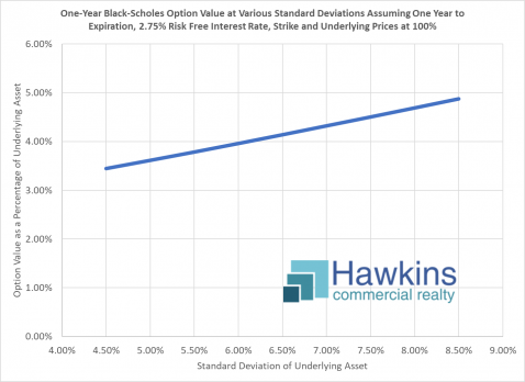
The chart above illustrates the price of a one year option at various SD assumptions. Here one can see that with the previously decided upon SD assumption of 6.5% annualized SD, a one year option would be just over 4% (4.14% to be exact), holding for other assumptions as noted. Thus, a one year option by this calculation should be $41,400 per million. Note how different assumptions affect this calculation, however. A higher SD assumption results in a higher price, a lower SD in a lower price.
With an option, the underlying asset may move in your favor or against. The ratio of the probability for or against is fixed at even odds. What is variable is the degree of the move. With move volatility, the potential for a larger move in your favor (or against) is higher. A larger potential move times a 50% probability of a move in favor of an option is greater than a smaller potential move times a 50% probability of a move in favor, thus the higher calculated value of the option.
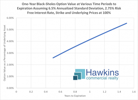
Time to expiration also, of course, affects the price. In the above chart, the other variables of SD and risk free interest rate are held constant as time to expiration is increased. This one is intuitive; more time costs more.
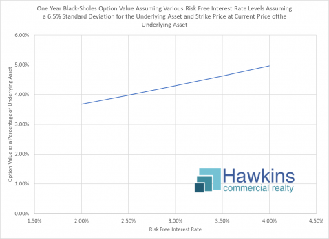
Finally, the is the input of risk free interest rates. As can be seen in the chart above, higher rates result in a higher calculated option price.
When one considers that an option buyer is participating in price movement of an asset that has not been purchased, then the time value of money on that preserved capital comes into play as a debit to the option buyer (offset by the credit of cost of money by not having to buy the asset). And, of course, as interest rates increase, so does the cost of money. Thus, the calculated value of an option increases as rates increase.
But Then the Norms…
Commercial property is commonly put under contract with a closing date two or three months in the future, sometimes more. These dates follow a due diligence period and sometimes financing or other contingency periods. While a property is under contract, and certainly while the owner has the contractual right to walk by way of the due diligence period language or otherwise, a contract is essentially an option on a property. Importantly, however, I’ve not seen this period considered as an option, and thus have not seen a option premium paid on any type of normal period. Thus, the norm is that this “option” is granted by sellers in return of undergoing a due diligence process.
On longer contracts the topic does not typically arise either. It is generally understood that for a seller to get his or her price, one is going to have to allow time for a buyer to get through one’s due diligence and other efforts and close. I believe a case can be made, however, that an option component should come into play as that period becomes particularly long. An option, after all, is a calculated fair value of the financial benefit of that option. To give it away in contract language without compensation is akin to allowing people to occupy rental property without (egads!) paying rent.
I have indeed seen a premium “paid” in the form of a price increased by the amount of calculated premium with that calculated premium being non-refundable. If you’ve read to this point, you might guess where I’ve seen this. If you guessed that it was a transaction I structured, you’re right. Doing it this way resulted in the same outcomes and allowed the structure to be put in place easily utilizing the standard FAR/BAR commercial contract.
So What’s the Bottom Line?
The bottom line is that a seller should be sure that he or she gets what is desired when entering into a contract to sell a property. If one is getting the price desired, and particularly if one is getting more, and is confident the buyer will close, that may be enough. However, as the length of time to closing and particularly the length of time for contingency periods to expires gets excessive, as one is less thrilled about the sales price, and/or as one is less confident that a buyer will close, collecting an option premium in the form of an amount above the price that is immediately non-refundable could be in order. As a rule of thumb, I use 4% of market value as the number, per year. That may be less than I calculated herein, but it is something in a world where most brokers give it no thought.
Perhaps move relevantly, when considering that one is essentially granting an option to a buyer in a contract with a due diligence period, it is important to know that a buyer is undergoing due diligence efforts to get to a close. Sussing out buyers that are not real is usually obvious to an experienced broker, but not to many sellers and frankly not to some brokers. This may be the most practical application of all this. In the bargain of executing a contract where a seller essentially grants an option and a buyer undergoes a due diligence process and otherwise moves toward a closing, a seller should make sure a buyer keeps up his or her side of the bargain.
Don’t rely on the above for investment related decisions. Instead consult with your accountant and other professional advisors.